Supplementary Material
Introduction
The concept of embedding random variables in Reproducing Kernel Hilbert Spaces (RKHS) has gained a lot of popularity and is one of the key aspects of many advanced forms of Bayesian inferencing routines and probabilistic programming. A very recent concept along these lines was introduced in [refer], which proposed an embedding for a function of random variables in RKHS. This was a very novel theoretical framework with very promising contributions like handling non-parametric forms of uncertainties, convergence with very low sample complexity etc., One of the key aspects of our proposed work is the mathematical workaround required to adopt this concept to a robotics scenario. In the current context, we attempt to solve a reactive navigation problem under uncertainty through a robust MPC framework. There is no assumption on the nature of the uncertainty involved here, it can be parametric or non parametric, Gaussian or non Gaussian. In short, we assume the source of uncertainty to be a black box model. This supplementary material focuses on the detailed derivations and implementations of the RKHS and GMM-KL divergence methods involved in the construction of our robust MPC framework.
Prerequisites
RKHS
RKHS is a Hilbert space with a positive definite function \( k(\cdot) :\ \mathbb{R}^n \times \mathbb{R}^N \to \mathbb{R} \) called the Kernel. Let, \( \textbf{x} \) denote an observation in physical space (say Euclidean). It is possible to embed this observation in the RKHS by defining the following kernel based function whose first argument is always fixed at \( \textbf{x} \). $$ \phi (\textbf{x}) = k(\textbf{x}, \cdot) \tag{1}$$
An attractive feature of RKHS is that it is endowed with an inner product which, in turn, can be used to model the distance between two functions in RKHS. Furthermore, the distance can be formulated in terms of kernel function in the following manner. $$ \langle \phi( \textbf{x}_i ), \phi( \textbf{x}_j ) \rangle = k(\textbf{x}_i, \textbf{x}_j) \tag{2}$$
The equation (2) is called the "kernel trick" and its strength lies in the fact that the inner product can be computed by only point wise evaluation of the kernel function.
Distribution Embedding of PVO
The important symbols that would be used in the rest of this material are summarized in the following table.
| \( \boldsymbol{\xi}_{t-1} \) | Robot state at time \( t-1 \) |
| \( {_j^o}\boldsymbol{\xi}_{t} \) | \( j^{th} \) Obstacle state at time \( t \) |
| \( \boldsymbol{\delta}_{t-1} \) | Control perturbation at time \( t-1 \) |
| \( \textbf{w}_{t-1} \) | \((\boldsymbol{\xi}_{t-1}, \boldsymbol{\delta}_{t-1} )\) |
| \( \textbf{u}_{t-1} \) | Control input at time \( t-1 \) |
| \( f_t^j(.) \) | VO constraint under deterministic conditions |
| \( P_{f_t^j}(\textbf{u}_{t-1}) \) | Distribution of \( f_t^j(.) \) under uncertainty |
| \( \eta \) | Chance constraint probability |
| \( P_{f_t^j}^{des} \) | Desired distribution |
| \( k(\cdot, \cdot) \) | Kernel function |
| \( \mu_{P_{f_t^j}} \) | RKHS embedding of \( P_{f_t^j} \) |
| \( \mu_{P_{f_t^j}^{des}} \) | RKHS embedding of the distribution \( P_{f_t^j}^{des} \) |
Let \( \textbf{w}^1_{t-1}, \textbf{w}^2_{t-1}, \ldots, \textbf{w}^n_{t-1} \) be samples drawn from a distribution corresponding to the uncertainty of the robot's state and control. Similarly, let \( {_j^o}\boldsymbol{\xi}_{t}^1, {_j^o}\boldsymbol{\xi}_{t}^2, \ldots, {_j^o}\boldsymbol{\xi}_{t}^n \) be samples drawn from the distribution corresponding to the uncertainty in the state of the obstacle. It is important to note here that the parametric forms of these distributions need not be known. Both these distributions (of the robot and the obstacle) can be represented in the RKHS through a function called the kernel mean, which is described as $$ \mu[\textbf{w}_{t-1}] = \sum^n_{p=1} \alpha_p k(\textbf{w}^p_{t-1}, \cdot) \tag{3}$$ $$ \mu[{_j^o}\boldsymbol{\xi}_{t}] = \sum^n_{q=1} \beta_q k({_j^o}\boldsymbol{\xi}_{t}^q, \cdot) \tag{4}$$ where \( \alpha_p \) is the weight associated with \( \textbf{w}^p_{t-1} \) and \( \beta_q \) is the weight associated with \( {_j^o}\boldsymbol{\xi}_{t}^q \). For example, if the samples are \( i.i.d. \), then \( \alpha_p = \frac{1}{n} \forall p \).
Following [refer], equation (4) can be used to embed functions of random variables like \( f^j_t(\textbf{w}_{t-1}, {_j^o}\boldsymbol{\xi}_{t}, \textbf{u}_{t-1}) \) shown in equation (5), where \( f_t^j \) is the VO constraint and \( \textbf{w}_{t-1}, {_j^o}\boldsymbol{\xi}_{t} \) are random variables with definitions taken from the above table. $$ \mu_{f^j_t}(\textbf{u}_{t-1}) = \sum^n_{p=1} \sum^n_{q=1} \alpha_p \beta_q k(f^j_t (\textbf{w}^p_{t-1}, {_j^o}\boldsymbol{\xi}_{t}^q, \textbf{u}_{t-1}), \cdot) \tag{5}$$
Similarly we can write the same for the samples for desired distribution, $$ \sum^{n_r}_{p=1} \sum^{n_o}_{q=1} \lambda_p \psi_q k(f^j_t (\widetilde{\textbf{w}^p}_{t-1}, \widetilde{{_j^o}\boldsymbol{\xi}_{t}^q}, \textbf{u}^{nom}_{t-1}), \cdot) $$ where \( \alpha_p, \beta_q, \lambda_p \) and \( \psi_q \) are the constants obtained from a reduced method that is explained in the paper.
An important point to notice from above is that for given samples \( \textbf{w}_{t-1}, {_j^o}\boldsymbol{\xi}_{t} \) the kernel mean is dependent on variable \( \textbf{u}_{t-1} \). The rest of the material focuses on the detailed derivation of the \( \mathcal{L}_{dist} \) used in our cost function to solve our robust MPC problem.
The proposed method has its foundations built by first posing the robust MPC as a moment matching problem (details of this can be found in Theorem 1 of the paper) and then describes a solution that is a work around based on the concept of embedding distributions in RKHS and Maximum Mean Discrepancy (MMD). Further insights on how MMD can act as a surrogate to the moment matching problem is described in Theorem 2 of the paper, which basically suggests that if two distributions \( P_{f^j_t} \) and \( P^{des}_{f^j_t} \), have their distributions embedded in RKHS for a polynomial kernel upto order \( d \), then decreasing the MMD distance becomes a way to match the first \( d \) moments of these distributions.
Using these insights, the following optimization problem was proposed in the paper. $$ \begin{align} \arg \min \rho_1 \mathcal{L}_{dist} + \rho_2 J(\textbf{u}_{t-1}) \\ \\ \mathcal{L}_{dist} = \Vert \mu_{{P}_{f^j_t}}(\textbf{u}_{t-1}) - \mu_{{P}^{des}_{f^j_t}} \Vert^2 \\ J(\textbf{u}_{t-1}) = \Vert\boldsymbol{\overline{\xi}}_{t} - \boldsymbol{\xi}_t^d\Vert_2^2 +\Vert \textbf{u}_{t-1}\Vert_2^2 \\ \\ \textbf{u}_{t-1} \in \mathcal{C} \end{align} \tag{6}$$
\begin{align} \Vert \mu_{{P}_{f^j_t}}(\textbf{u}_{t-1}) - \mu_{{P}^{des}_{f^j_t}} \Vert^2 & = \langle \mu_{{P}_{f^j_t}}(\textbf{u}_{t-1}), \mu_{{P}_{f^j_t}}(\textbf{u}_{t-1}) \rangle - 2 \langle \mu_{{P}_{f^j_t}}(\textbf{u}_{t-1}), \mu_{{P}^{des}_{f^j_t}} \rangle + \langle \mu_{{P}^{des}_{f^j_t}}, \mu_{{P}^{des}_{f^j_t}} \rangle \\ & = \langle \sum^n_{p=1} \sum^n_{q=1} \alpha_p \beta_q k(f^j_t (\textbf{w}^p_{t-1}, {_j^o}\boldsymbol{\xi}_{t}^q, \textbf{u}_{t-1}), \cdot), \sum^n_{p=1} \sum^n_{q=1} \alpha_p \beta_q k(f^j_t (\textbf{w}^p_{t-1}, {_j^o}\boldsymbol{\xi}_{t}^q, \textbf{u}_{t-1}), \cdot) \rangle \\ & - 2 \langle \sum^n_{p=1} \sum^n_{q=1} \alpha_p \beta_q k(f^j_t (\textbf{w}^p_{t-1}, {_j^o}\boldsymbol{\xi}_{t}^q, \textbf{u}_{t-1}), \cdot), \sum^{n_r}_{p=1} \sum^{n_o}_{q=1} \lambda_p \psi_q k(f^j_t (\widetilde{\textbf{w}^p}_{t-1}, \widetilde{{_j^o}\boldsymbol{\xi}_{t}^q}, \textbf{u}^{nom}_{t-1}), \cdot) \rangle \\ & + \langle \sum^{n_r}_{p=1} \sum^{n_o}_{q=1} \lambda_p \psi_q k(f^j_t (\widetilde{\textbf{w}^p}_{t-1}, \widetilde{{_j^o}\boldsymbol{\xi}_{t}^q}, \textbf{u}^{nom}_{t-1}), \cdot), \sum^{n_r}_{p=1} \sum^{n_o}_{q=1} \lambda_p \psi_q k(f^j_t (\widetilde{\textbf{w}^p}_{t-1}, \widetilde{{_j^o}\boldsymbol{\xi}_{t}^q}, \textbf{u}^{nom}_{t-1}), \cdot) \rangle \end{align}
Using kernel trick, the above expression can be reduced to \begin{align} \Vert \mu_{{P}_{f^j_t}}(\textbf{u}_{t-1}) - \mu_{{P}^{des}_{f^j_t}} \Vert^2 & = \ \textbf{C}_{\alpha \beta} \textbf{K}_{f^j_t f^j_t} \textbf{C}_{\alpha \beta}^T \ - \ 2 \textbf{C}_{\alpha \beta} \textbf{K}_{f^j_t \widetilde{f^j_t}} \textbf{C}_{\lambda \psi}^T \ + \ \textbf{C}_{\lambda \psi} \textbf{K}_{\widetilde{f^j_t} \widetilde{f^j_t}} \textbf{C}_{\lambda \psi}^T \end{align} \begin{aligned} \textbf{C}_{\alpha \beta} & = \ \begin{bmatrix} \alpha_1 \beta_1 & \alpha_2 \beta_2 & \cdots & \alpha_n \beta_n \end{bmatrix}_{1 \times n^2} \\ \textbf{C}_{\lambda \psi} & = \ \begin{bmatrix} \lambda_1 \psi_1 & \lambda_2 \psi_2 & \cdots & \lambda_n \psi_n \end{bmatrix}_{1 \times n_r n_o} \\ \textbf{K}_{f^j_t f^j_t} & = \ \begin{bmatrix} \textbf{K}^{11}_{f^j_t f^j_t} & \textbf{K}^{12}_{f^j_t f^j_t} & \cdots & \textbf{K}^{1n}_{f^j_t f^j_t} \\ \textbf{K}^{21}_{f^j_t f^j_t} & \textbf{K}^{22}_{f^j_t f^j_t} & \cdots & \textbf{K}^{2n}_{f^j_t f^j_t} \\ \vdots & \vdots & \ddots & \vdots \\ \textbf{K}^{n1}_{f^j_t f^j_t} & \textbf{K}^{n2}_{f^j_t f^j_t} & \cdots & \textbf{K}^{nn}_{f^j_t f^j_t} \\ \end{bmatrix} \\ \textbf{K}^{ab}_{f^j_t f^j_t} & = \ \begin{bmatrix} k(f^j_t (\textbf{w}^a_{t-1}, {_j^o}\boldsymbol{\xi}_{t}^1, \textbf{u}_{t-1}), f^j_t (\textbf{w}^b_{t-1}, {_j^o}\boldsymbol{\xi}_{t}^1, \textbf{u}_{t-1})) & \cdots & k(f^j_t (\textbf{w}^a_{t-1}, {_j^o}\boldsymbol{\xi}_{t}^1, \textbf{u}_{t-1}), f^j_t (\textbf{w}^b_{t-1}, {_j^o}\boldsymbol{\xi}_{t}^n, \textbf{u}_{t-1})) \\ \vdots & \ddots & \vdots \\ k(f^j_t (\textbf{w}^a_{t-1}, {_j^o}\boldsymbol{\xi}_{t}^n, \textbf{u}_{t-1}), f^j_t (\textbf{w}^b_{t-1}, {_j^o}\boldsymbol{\xi}_{t}^1, \textbf{u}_{t-1})) & \cdots & k(f^j_t (\textbf{w}^a_{t-1}, {_j^o}\boldsymbol{\xi}_{t}^n, \textbf{u}_{t-1}), f^j_t (\textbf{w}^b_{t-1}, {_j^o}\boldsymbol{\xi}_{t}^n, \textbf{u}_{t-1})) \end{bmatrix}_{n \times n} \\ \textbf{K}_{f^j_t \widetilde{f^j_t}} & = \ \begin{bmatrix} \textbf{K}^{11}_{f^j_t \widetilde{f^j_t}} & \textbf{K}^{12}_{f^j_t \widetilde{f^j_t}} & \cdots & \textbf{K}^{1n_r}_{f^j_t \widetilde{f^j_t}} \\ \textbf{K}^{21}_{f^j_t \widetilde{f^j_t}} & \textbf{K}^{22}_{f^j_t \widetilde{f^j_t}} & \cdots & \textbf{K}^{2n_r}_{f^j_t \widetilde{f^j_t}} \\ \vdots & \vdots & \ddots & \vdots \\ \textbf{K}^{n1}_{f^j_t \widetilde{f^j_t}} & \textbf{K}^{n2}_{f^j_t \widetilde{f^j_t}} & \cdots & \textbf{K}^{nn_r}_{f^j_t \widetilde{f^j_t}} \\ \end{bmatrix} \\ \textbf{K}^{ab}_{f^j_t \widetilde{f^j_t}} & = \ \begin{bmatrix} k(f^j_t (\textbf{w}^a_{t-1}, {_j^o}\boldsymbol{\xi}_{t}^1, \textbf{u}_{t-1}), f^j_t (\widetilde{\textbf{w}^b}_{t-1}, \widetilde{{_j^o}\boldsymbol{\xi}_{t}^1}, \textbf{u}^{nom}_{t-1})) & \cdots & k(f^j_t (\textbf{w}^a_{t-1}, {_j^o}\boldsymbol{\xi}_{t}^1, \textbf{u}_{t-1}), f^j_t (\widetilde{\textbf{w}^b}_{t-1}, \widetilde{{_j^o}\boldsymbol{\xi}_{t}^{n_o}}, \textbf{u}^{nom}_{t-1})) \\ \vdots & \ddots & \vdots \\ k(f^j_t (\textbf{w}^a_{t-1}, {_j^o}\boldsymbol{\xi}_{t}^n, \textbf{u}_{t-1}), f^j_t (\widetilde{\textbf{w}^b}_{t-1}, \widetilde{{_j^o}\boldsymbol{\xi}_{t}^1}, \textbf{u}^{nom}_{t-1})) & \cdots & k(f^j_t (\textbf{w}^a_{t-1}, {_j^o}\boldsymbol{\xi}_{t}^n, \textbf{u}_{t-1}), f^j_t (\widetilde{\textbf{w}^b}_{t-1}, \widetilde{{_j^o}\boldsymbol{\xi}_{t}^{n_o}}, \textbf{u}^{nom}_{t-1})) \end{bmatrix}_{n \times n_o} \end{aligned}
Implementation
All the above mentioned matrix operations can be parallelised using a GPU. We used pytorch to evaluate the embeddings and MMD distances on the GPU. It should be noted that we were able to boost the performance using GPU because of the nature of the formulation. On the other hand, GMM-KL divergence based approach relies on fitting a GMM and estimating the density values of the fitted GMM. If we were to parallelise GMM-KL divergence approach using a GPU, the only possible place to do this would be the estimation of values of PDF of the samples. The overhead involved in copying the array between CPU and GPU buffers and also in serialising the arguments which will be passed to the worker pool (this worker pool will evaluate the PDF values) will make the GPU implementation of GMM-KL divergence approach less efficient than that of the same implemented on multiple CPU sub-processes. This is not the case with RKHS based approach because we copy the \( f^j_t \) values once into the GPU buffers and rest of the compution happens completely on GPU (basically the total amount of uploads and downloads from GPU memory will be far lesser for RKHS based approach).
All the CPU based matrix/vector operations were carried out using numpy. For parallel evaluation of the coefficients of \( f_t^j \) (equation (3) in the paper) and PDF values for KLD, we used python's multiprocessing library. The numpy library we used was compiled with support for Intel MKL.
The computation times for both the approaches are reported in table 2 of the paper.
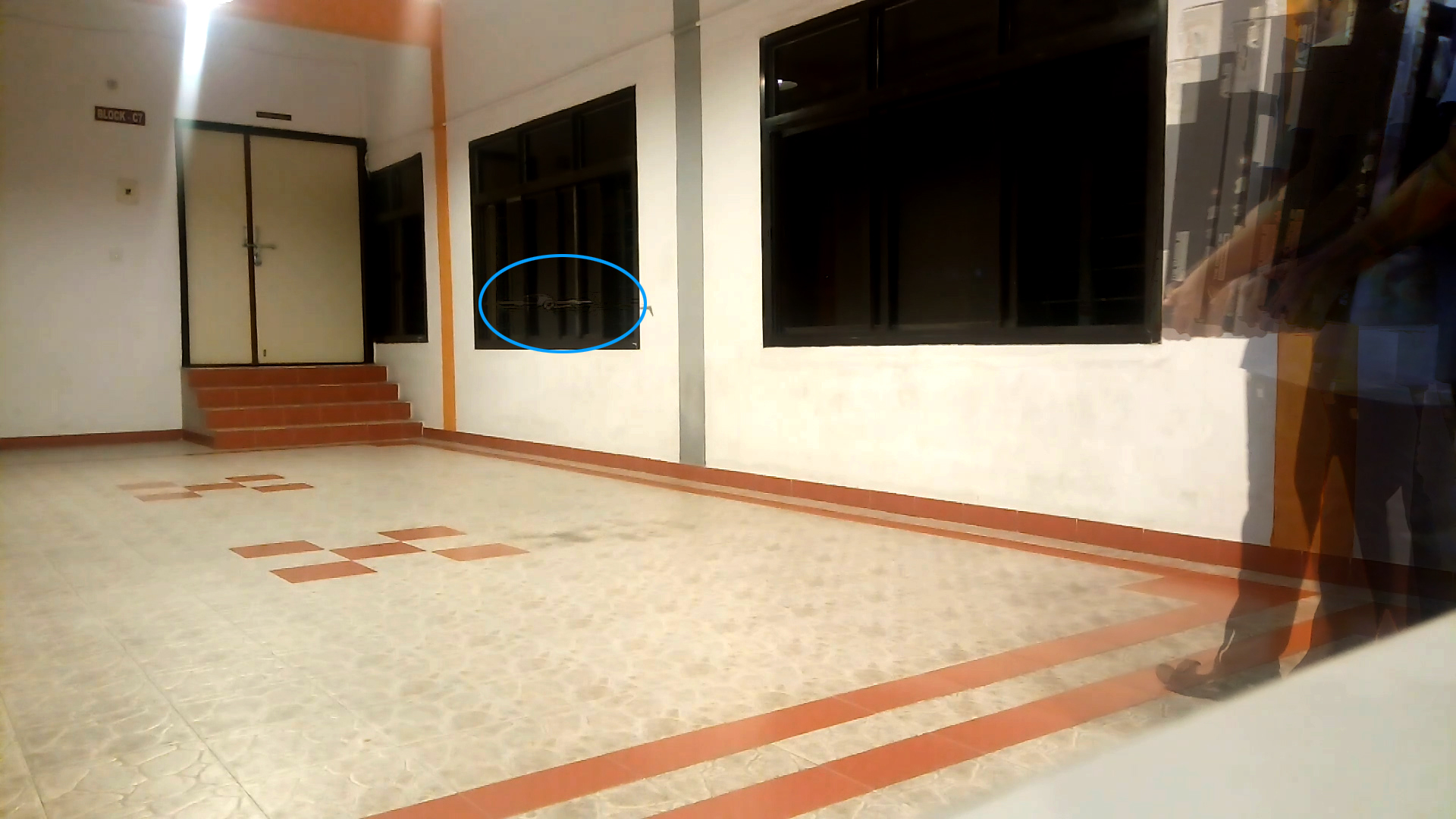
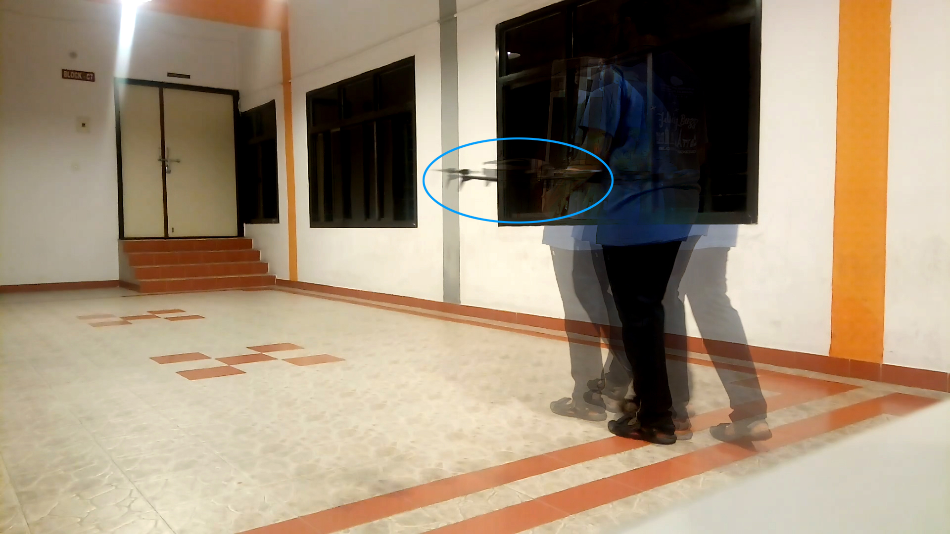
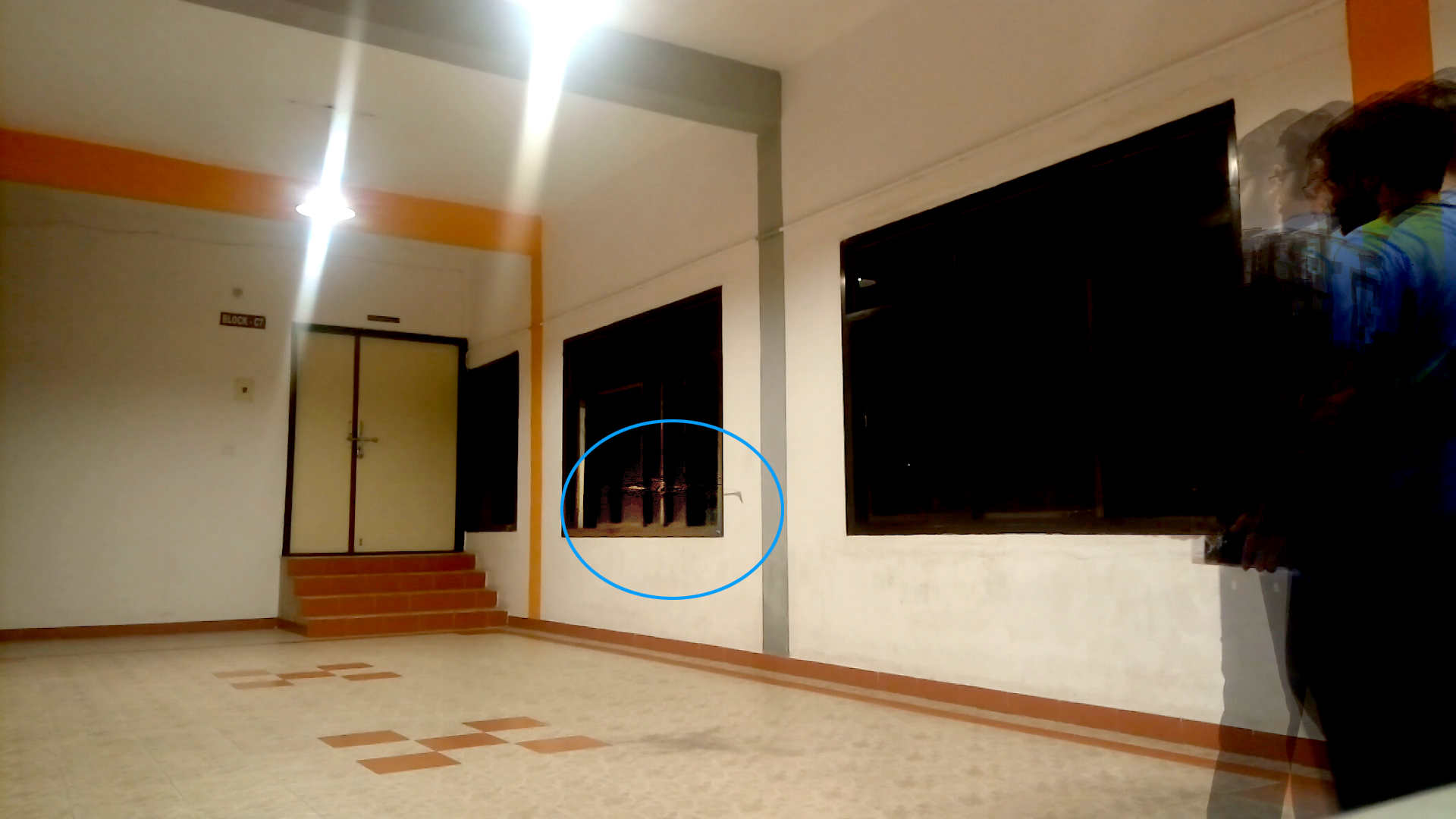
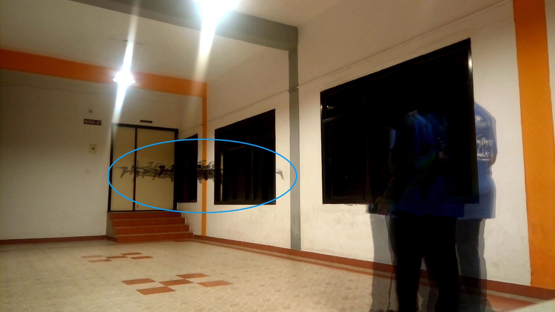
Interpretation of Real Runs
The RKHS framework was implemented on a Bebop drone equipped with a monocular camera. A person walking withan April tag marker in front of him constitute the moving object. Distance and bearing to the marker is computed using the April Tag library from which the velocity information is obtained. The state and velocity of the drone is obtained from the on board odometry (estimated using an onboard IMU). The state, velocity, control and perception/measurement noise distributions were computed through a non-parametric Pearson fit over experimental data obtained over multiple runs. A number of experimental runs, totally 15, were performed to evaluate the RKHS method. We show that increasing the power of the polynomial kernel, d, decreases the overlap of the samples of the robot and the obstacle leading to more conservative maneuvers.
d = 1
d = 1
d = 3
d = 3
The below figures further analyze the results of the real run. The robot samples are represented using translucent blue circles while the obstacle samples are represented using translucent yellow circles. The means of the robot and the obstacl are represented using opaque blue and yellow circles respectively.
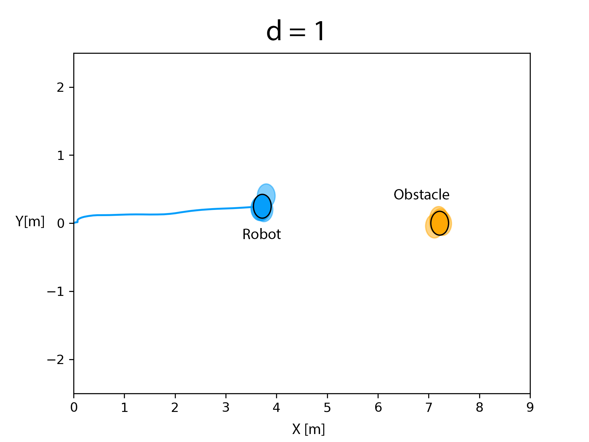
Before obstacle entered the critical distance. Critical distance is when the robot starts avoiding the obstacle.
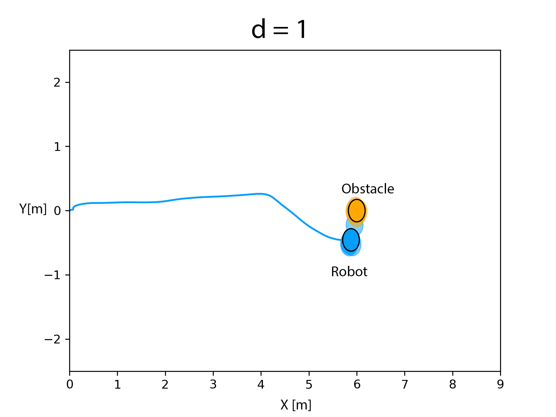
After the obstacle entered the critical distance, the robot adopts the maneuver obtained by evaluating the optimization routine proposed in equation (6). The kernel matrices were evaluated for a polynomial order of d = 1. It could be observed that there is a considerable amount of overlap between the samples of the robot and obstacle.
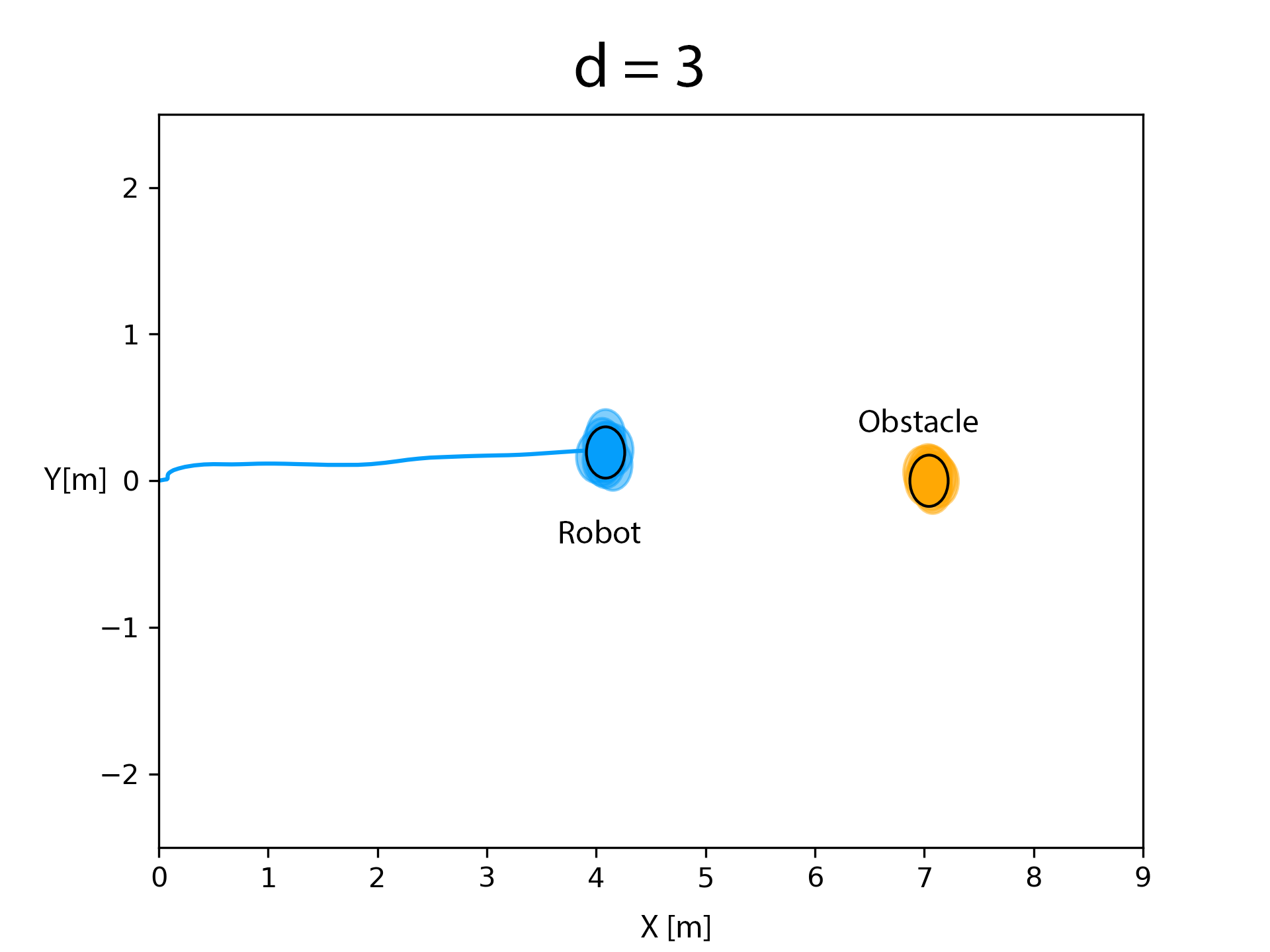
Before obstacle entered the critical distance. Critical distance is when the robot starts avoiding the obstacle.
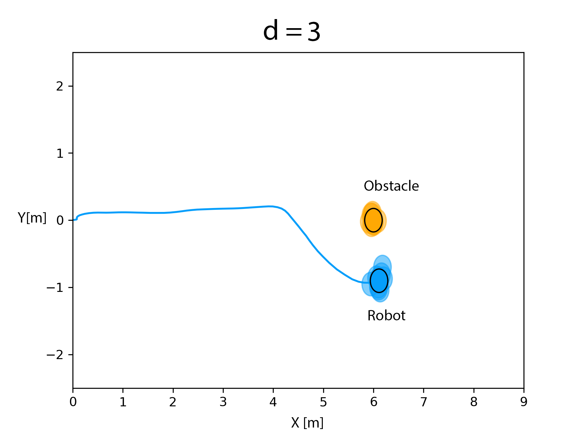
After obstacle entered the critical distance, the optimization routine in equation (6) was evaluated by computing the kernel matrices for d = 3. It could be observed that there is almost no overlap.
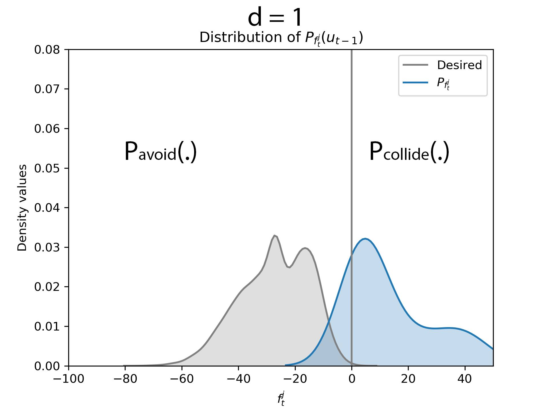
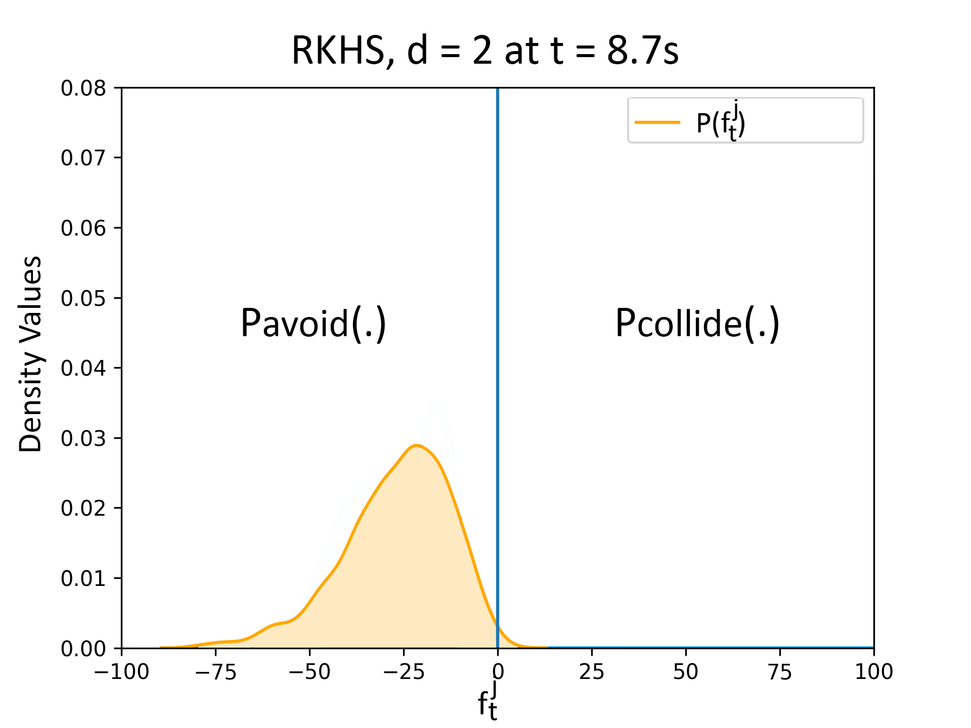
Distribution of \( f^j_t \) before the obstacle entered the critical distance. Critical distance is when the robot starts avoiding the obstacle.
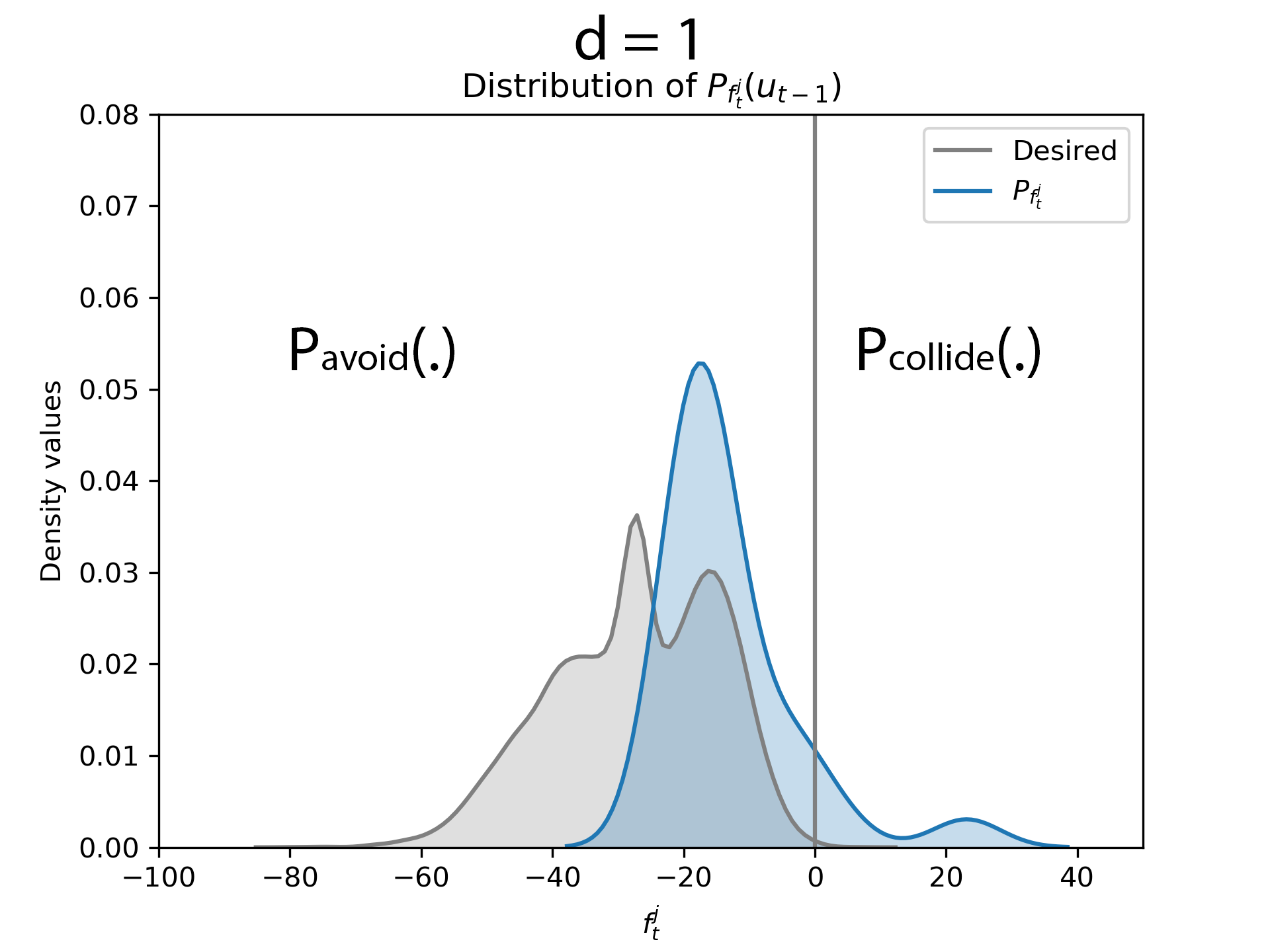
After the obstacle entered the critical distance, we evaluate the kernel matrices for d = 1 and it could be observed that a portion of the right tail of \( P_{f^j_t} \) is on the right side of zero and the area of overlap with the desired distribution is lesser compared to d = 3 case.
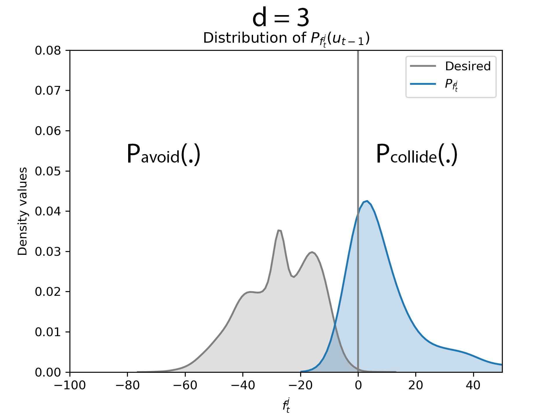
Before obstacle entered the critical distance. Critical distance is when the robot starts avoiding the obstacle.
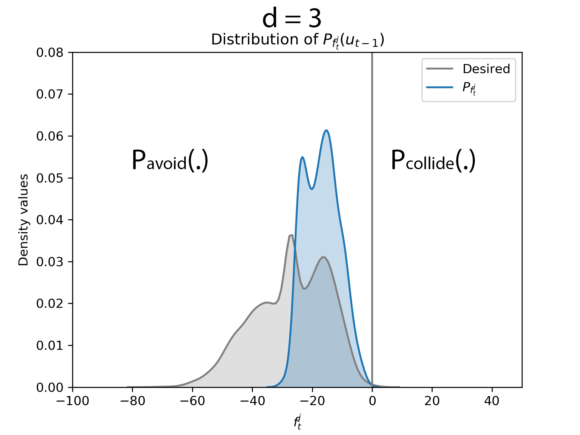
After obstacle entered the critical distance, we evaluate the kernel matrices for d = 3 and it could be noticed that almost the entire distribution is on the left side of zero and the area of overlap of \( P_{f^j_t} \) and the desired distribution is higher.
Guarantees on Safety
Both our GMM-KLD and RKHS based approach works with only sample level information without assuming any parametric form for the underlying distribution. Thus, the performance guarantees on safety depends on the following aspects. First, on how well are we modeling the distribution of our collision avoidance function (PVO) for a given finite sample size. Second, does our modeling improve as the samples increase: a property popularly known as consistency in estimation. Third, can we tune our model to produce diverse trajectories with varied probability of avoidance in line with the original robust MPC formulation. The discussion regarding the consistency, has been addressed in section 3.7 of the paper. The third question has already been addressed in Remark 2 in the paper and additional results validating this are provided in the following subsections. Moreover, first two questions about GMM-KLD based approaches have already been established in the existing literature [refer], [refer].
Trajectory Tuning
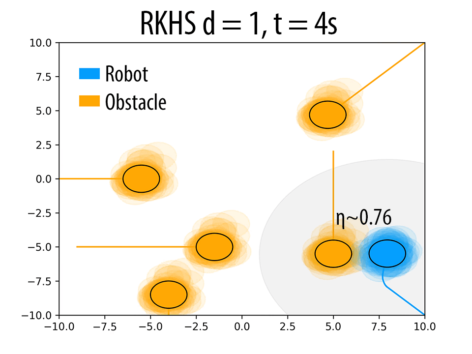
As mentioned in Remark 2 of the paper and also validated in the results Section 4 of the paper, the polynomial kernel order \( d \) can be used to produce trajectories with different probability of collision avoidance \( \eta \). Herein, we presents some additional results to back our claims. The following figure summarizes these results. As \( d \) increases, the robot seeks to maintain higher clearance from the obstacles.
 (a)
(a)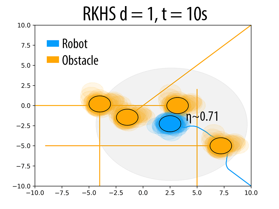 (b)
(b)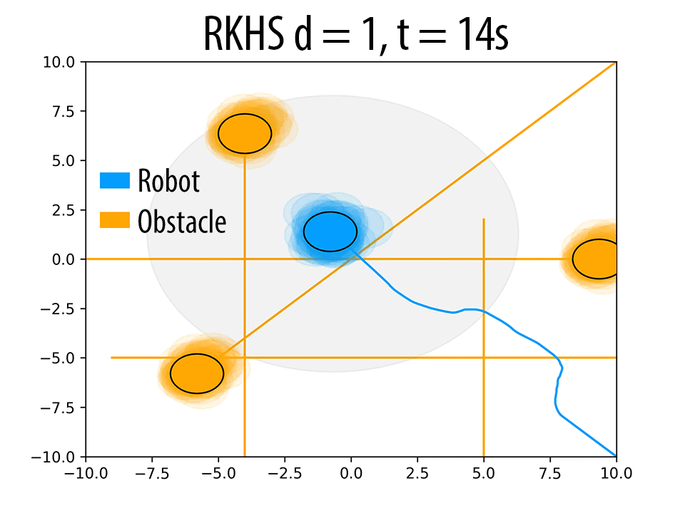 (c)
(c)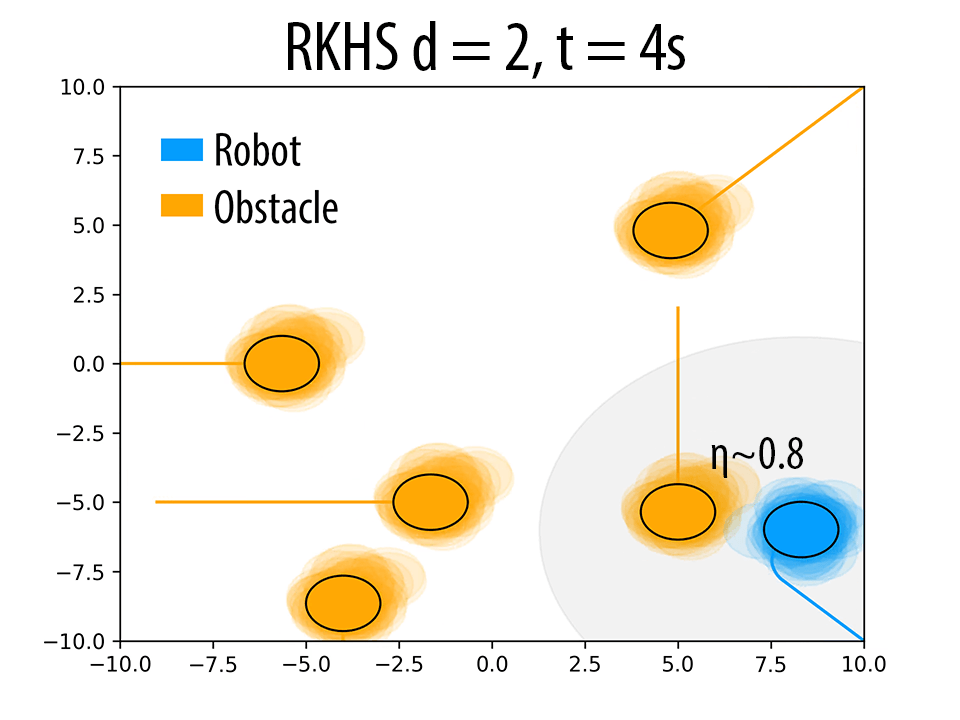 (d)
(d)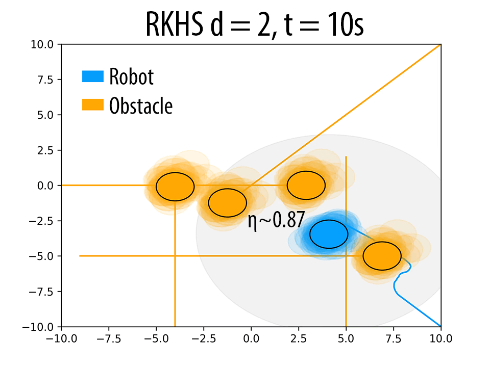 (e)
(e)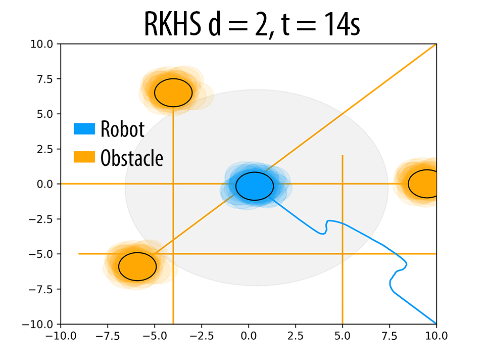 (f)
(f)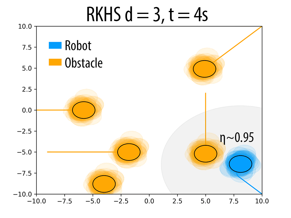 (g)
(g)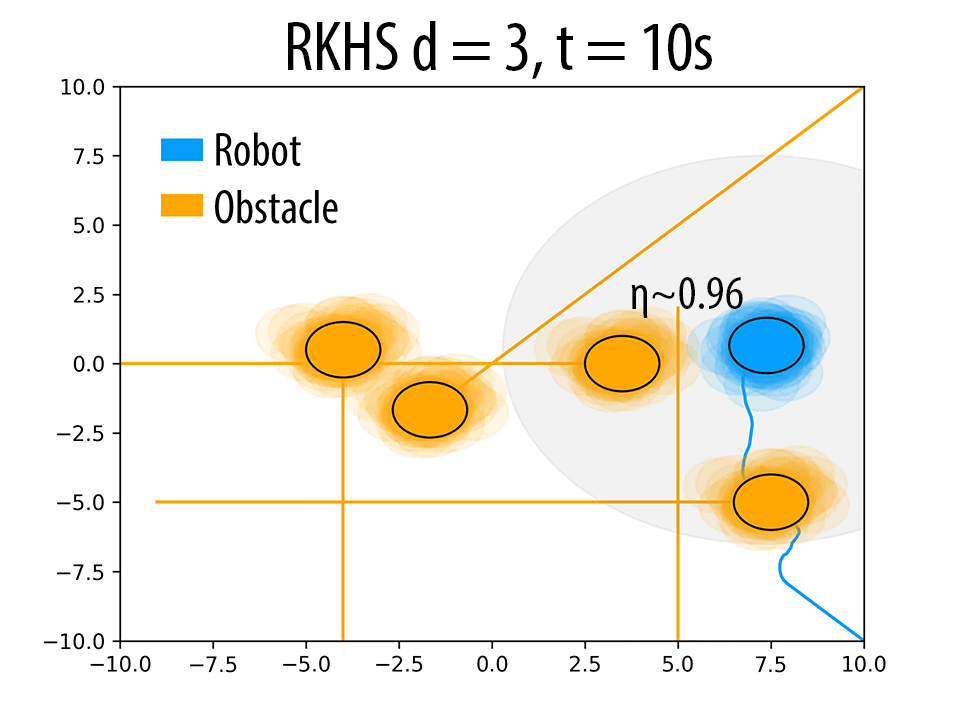 (h)
(h)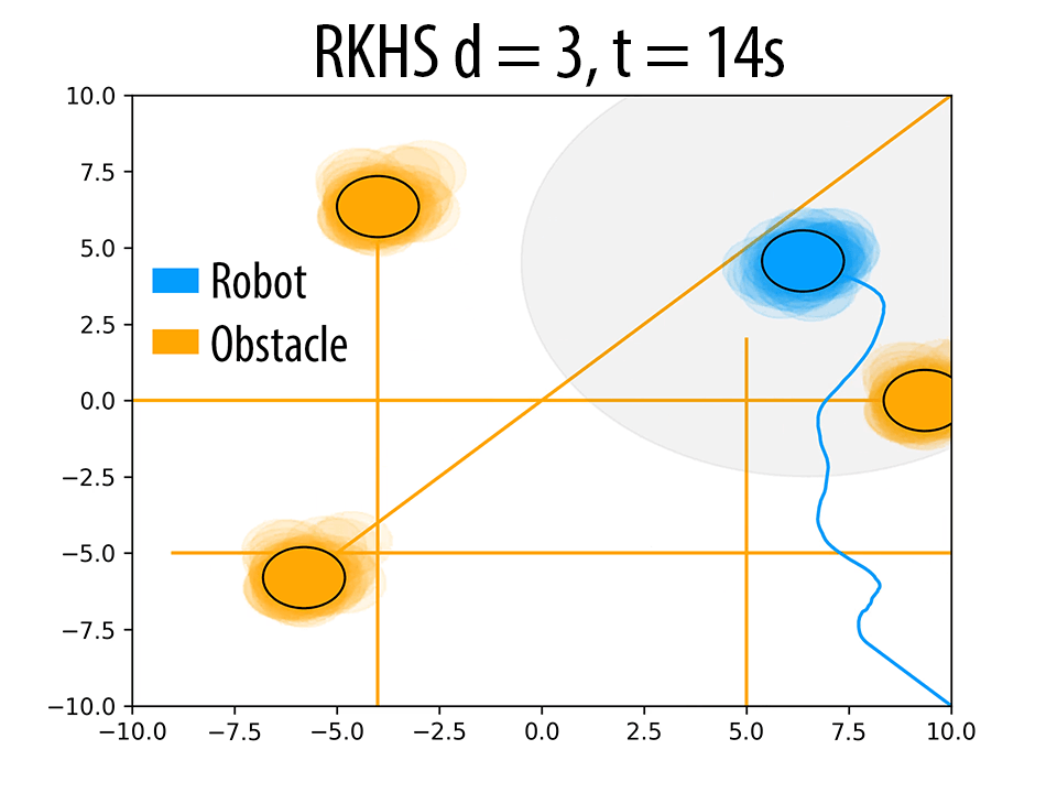 (i)
(i)Effect of \( d \) on the trajectory of the robot. \( \eta \) increases with increase in \( d \). In figures (a),(d) and (g) (at t = 4s), for a similar configuration, with increasing \( d \), the number of samples of robot and obstacle that overlap decreases, thereby resulting in higher \( \eta \) values. Similar trend is observed in b, e and h (at t = 10s). The different trajectories resulted due to different \( d \) values are shown in figures (c),(f) and (i) (at t = 14s).
Comparisons with the existing methods in the literature
Linearized constraints with Gaussian approximation of uncertainty
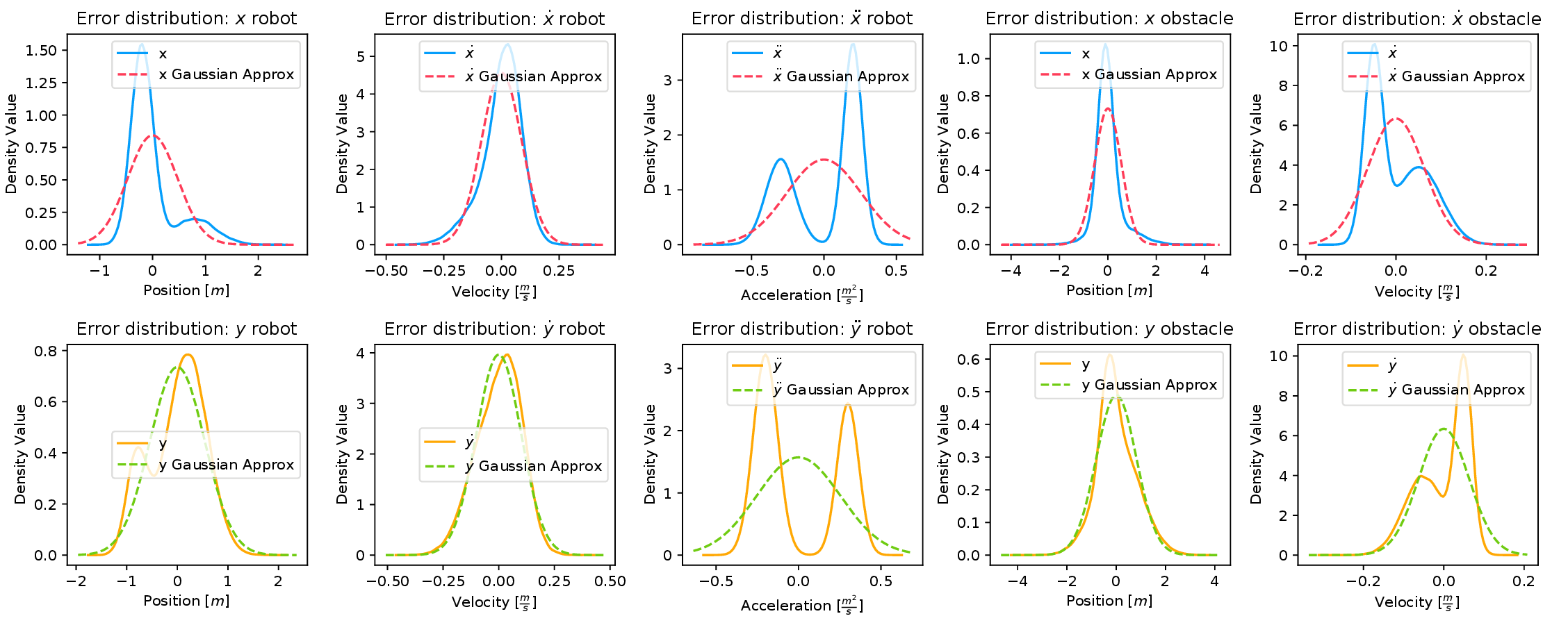
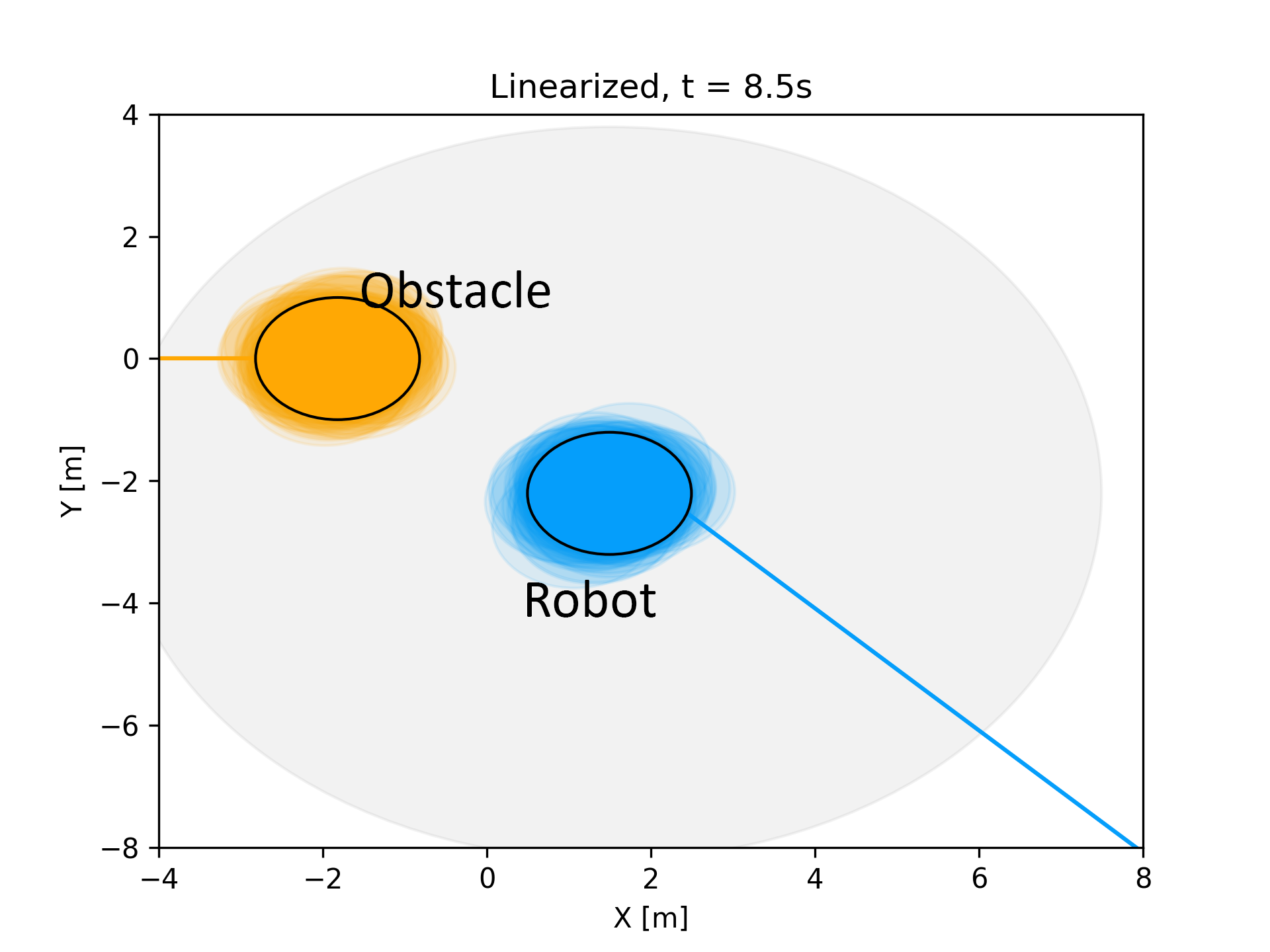
For this comparison, we first fit a Gaussian to the error distribution (shown in the above figure) and consequently, approximate \( \textbf{w}_{t-1},\ {_{j}^{o}}\boldsymbol{\xi}_{t}\) as Gaussian random variables. We subsequently compute an affine approximation of\( f_t^j(.)\) which we denote as \( \hat{f}_t^j(.)\) by linearizing with respect to \( \textbf{w}_{t-1}\) and \( {_{j}^{o}}\boldsymbol{\xi}_{t}\) . Note that the linearization is with respect to random variables and not \( \textbf{u}_{t-1}\). \( \hat{f}_t^j(.)\) is still non-linear in\( \textbf{u}_{t-1}\) But nevertheless,\( P_{\hat{f}_t^j}(\textbf{u}_{t-1})\) takes a Gaussian form [refer]. We can now easily adopt sampling based procedure to obtain the control \( \textbf{u}_{t-1}\) such that \( P({\hat{f}^j_t(.)}\leq0)\geq\eta\) is satisfied, where \( \eta\) is the probability of collision avoidance. The following figure summarizes the results. The subfigure (a) in the following figure shows a robot in imminent collision with a dynamic obstacle. The true distribution\( P_{f_t^j}(\textbf{u}_{t-1})\) and the Gaussian approximation\( P_{\hat{f}_t^j}(\textbf{u}_{t-1})\) for the computed control input is shown in the subfigure (b) of the following figure. As shown, the Gaussian approximation lies completely to the left of \( f_t^j=0\) , line indicating collision avoidance with a very high probability for the computed control input. However, in reality true distribution has a significant mass to the right of \( f_t^j=0\) indicating a risk of collision. Thus, this experiment clearly shows that the Gaussian approximation results in a collision avoidance algorithm that is not robust.
 (a)
(a)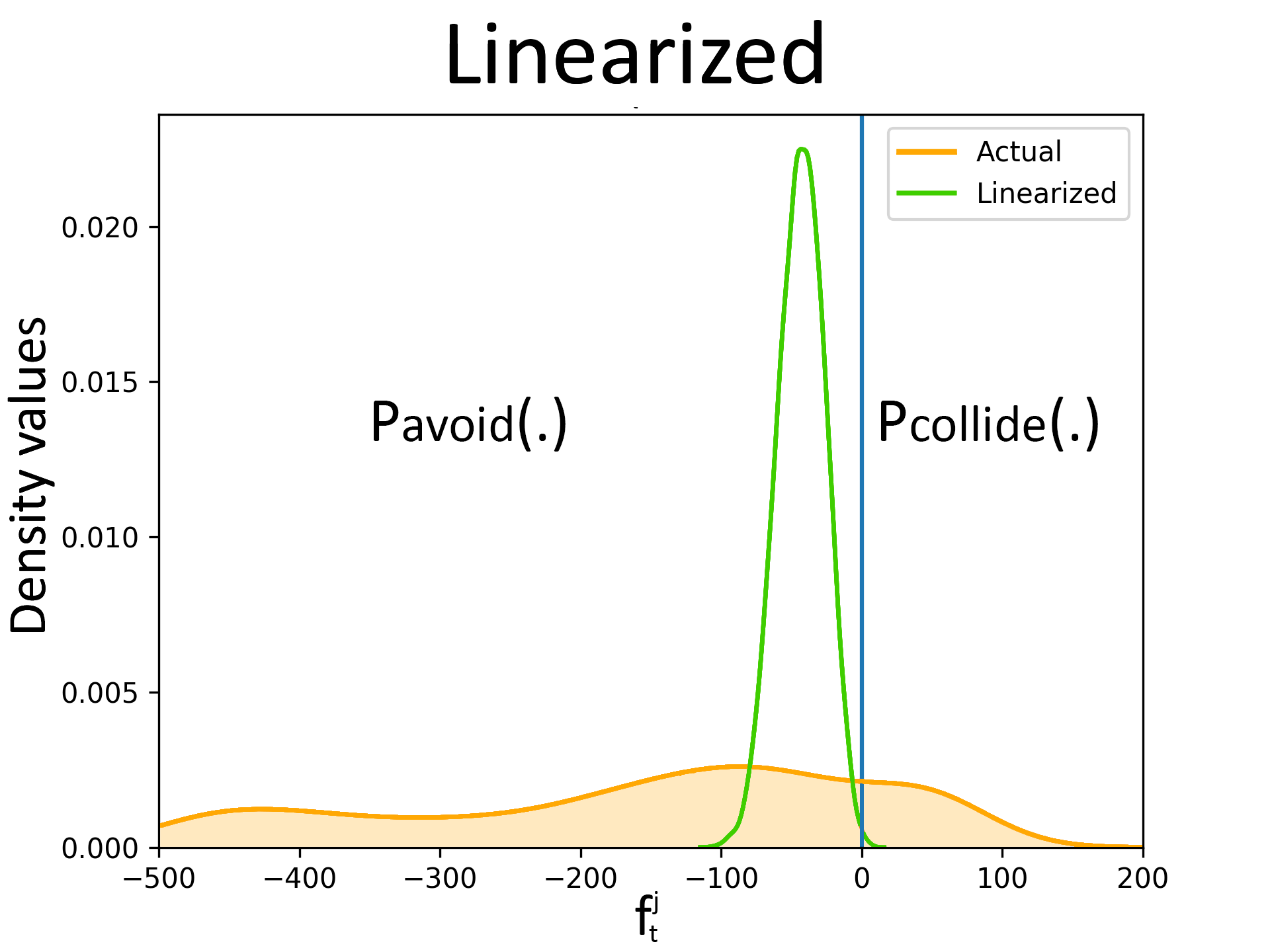 (b)
(b)We show the results for linearization+Gaussian approximation approach for the one obstacle benchmark in Fig. 4 of the paper. The figure on the left (a) shows the distribution plot for \( P_{fˆj_t}(ut−1) \) while the figure on the right (b) shows the robot (blue), obstacle (yellow), sensing range (gray). At t = 8.5s, a considerable portion of the true distribution of \( P_{fˆj_t} \) is on the right of zero (which means high probability of collision) while the Gaussian approximation \( P_{fˆj_t} \) is completely on the left side of the zero line. This implies that \( P_{fˆj_t} \) is a misrepresentation of \( P_{fˆj_t} \). The same can be inferred from the figure where the robot seems to be on a collision course with the obstacle.
The following figure summarizes the collision avoidance results obtained with our RKHS based approach. As clearly shown, we can compute a control input which brings the true distribution \( P_{f_t^j}(\textbf{u}_{t-1})\) to the left of \( f_t^j=0\) .
 (a)
(a)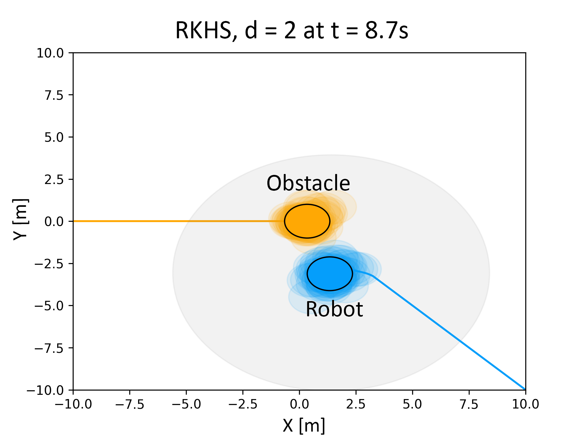 (b)
(b)The figure on the left shows the distribution plots for \( P_{fˆj_t} \) while the figure on the right shows the robot (blue), obstacle (yellow), sensing range (gray). Unlike the case of the linearized constraints, the robot starts avoiding the obstacle in the RKHS based approach.
Comparison with Gaussian approximation + exact surrogate based approach
In this approach, we first fit a Gaussian to the error distribution (the same error distributions shown in the previous section) and consequently, approximate \( \textbf{w}_{t-1}, {_{j}^{o}}\boldsymbol{\xi}_{t} \) as Gaussian random variables. Subsequently, we replace the chance constraints with the following surrogate used in works like [refer], [refer], [refer].
$$ \begin{align} E[f_t^j(.)]+\epsilon\sqrt{Var[f_t^j(.)]}\leq 0, \eta\geq \frac{\epsilon^2}{1+\epsilon^2} \end{align} \tag{7} $$where, \( E[f_t^j(.)] \), \( Var[f_t^j(.)] \) respectively represent the expectation and variance of \( f_t^j(.) \) taken with respect to random variables \( \textbf{w}_{t-1}, {_{j}^{o}}\boldsymbol{\xi}_{t} \). It can be shown that the satisfaction of equation (7) ensures the satisfaction of chance constraints with confidence \( \eta\geq \frac{\epsilon^2}{1+\epsilon^2} \). Note that for Gaussian uncertainty, \( E[f_t^j(.)] \), \( Var[f_t^j(.)] \) have a closed form expression. We henceforth call this approach EV-Gauss.
An example simulation is presented in the following figure where a robot tries to avoid three dynamic obstacles. Two different instances of this simulation were performed, that corresponded to robot requiring to avoid the obstacles with atleast \( \eta=0.60 \) and \( \eta = 0.80 \).
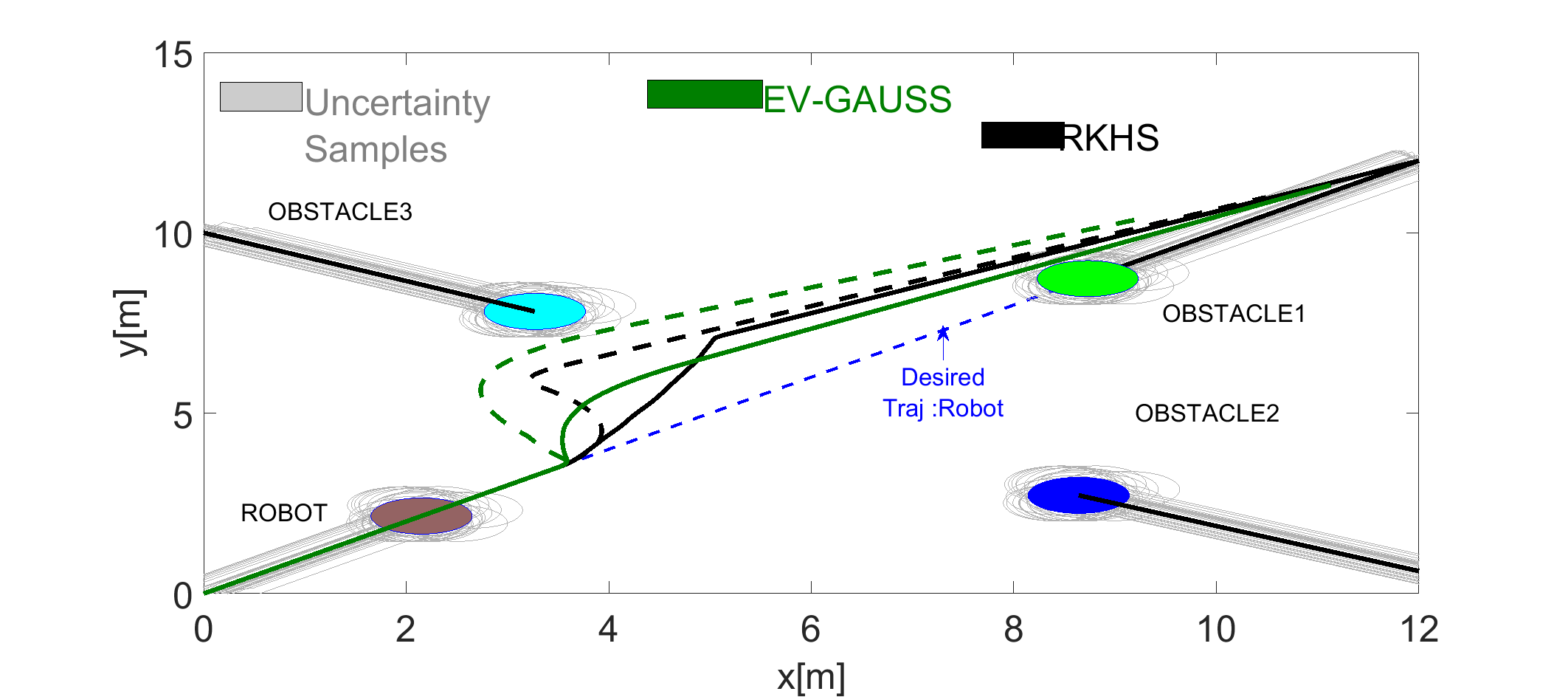
Trajectory comparison obtained with our proposed RKHS based approach and EV Gauss. The solid lines represent trajectories for \( \eta=0.60 \) and the dotted lines correspond to \( \eta=0.80 \). As shown, EV-Gauss approach leads to higher deviation from the desired trajectory.
The following figure performs the validation by showing the plot of actual \( \eta \) over time obtained through Monte-Carlo sampling. As can be seen, at low \( \eta \), both EV-Gauss and our RKHS based algorithm result in similar \( \eta \) profile. However, at high \( \eta \) (subfigure (b)), EV-Gauss performs unreliably and does not maintain the required \( \eta \) for the entire trajectory run. This can be attributed to the Gaussian approximation of the uncertainty used by EV-Gauss.
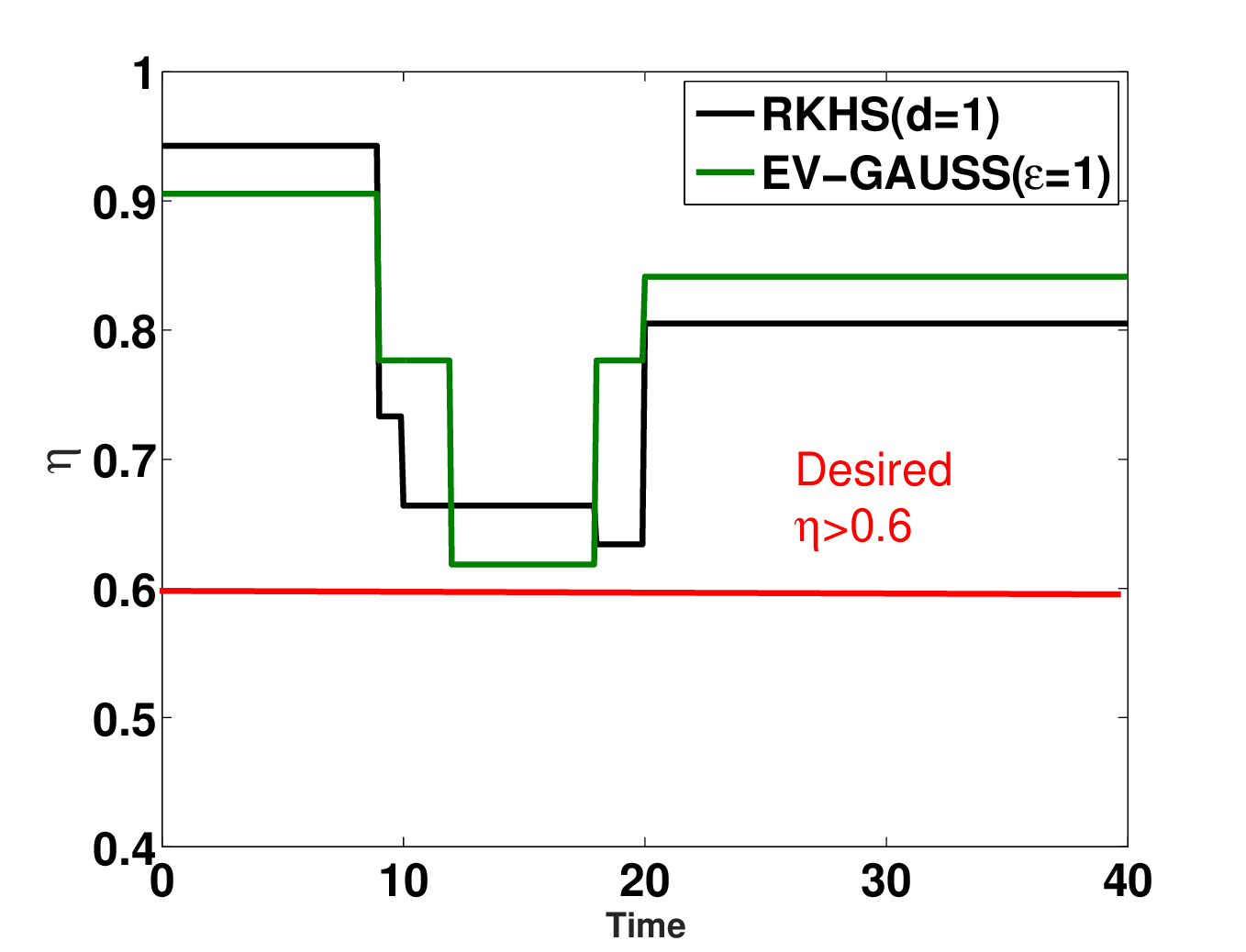 (a)
(a)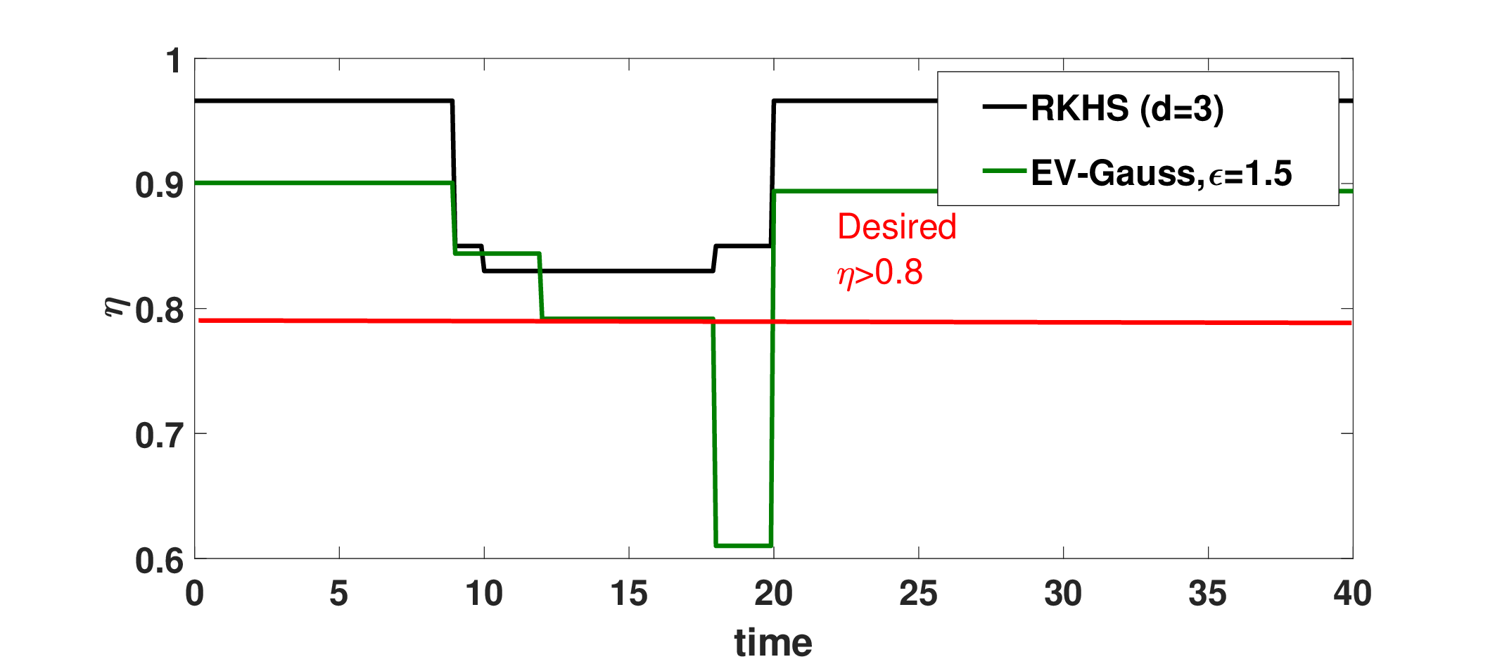 (b)
(b)Confidence plots for EV Gauss based approach. At high η (subfigure (b)) the EV Gauss method fails to maintain the minimum confidence required, while RKHS based method performs more reliably.
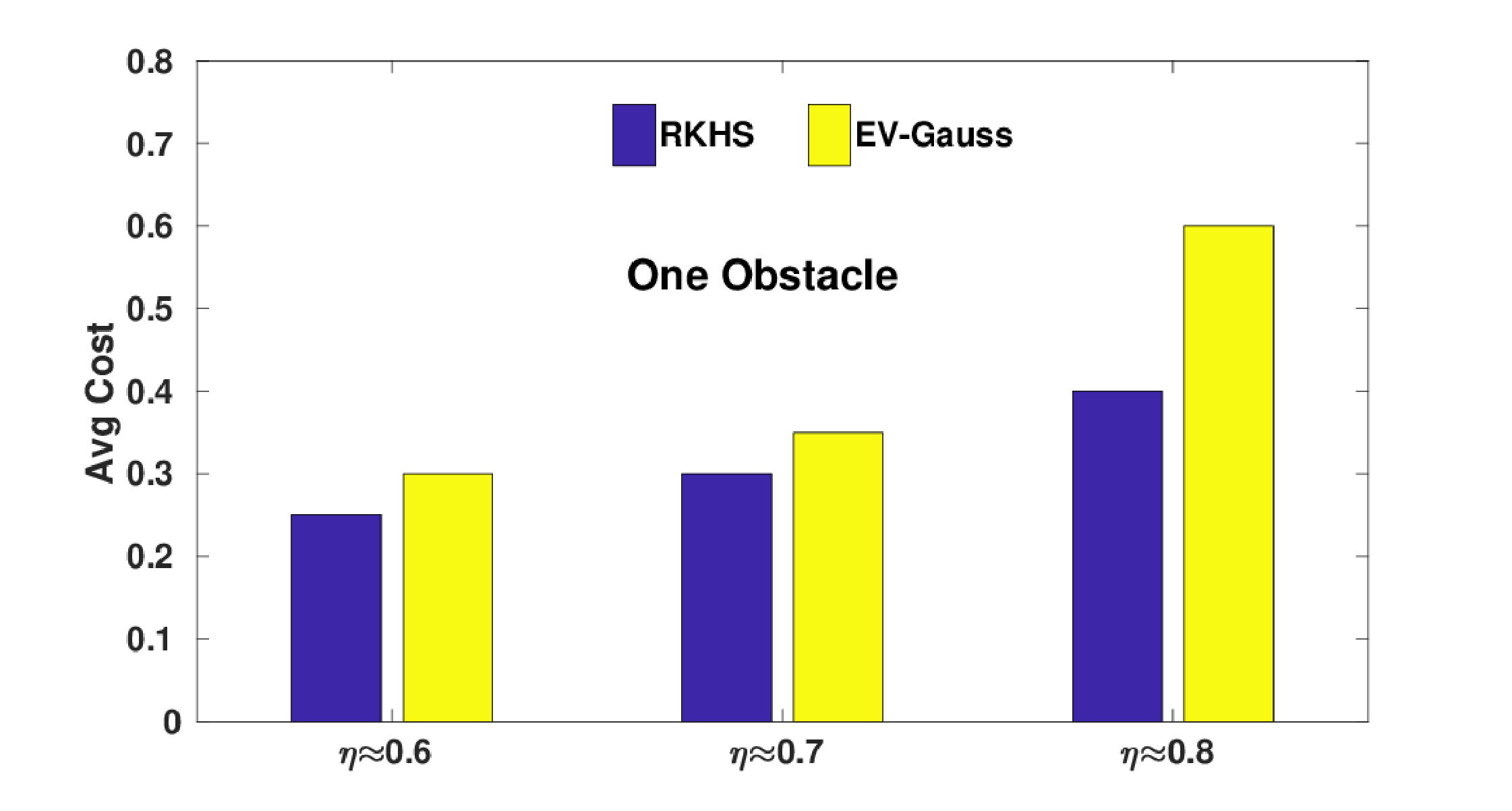
The following figure presents the comparison of average optimal cost obtained with EV-Gauss and our RKHS based approach over 10 simulation instances with varied number of obstacles. Note that, the optimal cost is a combination of norm of the tracking error and magnitude of the control inputs used. To put it quantitatively, EV-Gauss resulted in 27% larger cost than our RKHS approach \( \eta=0.60 \). This number jumps to 34% and 40% at \( \eta=0.70 \) and \( \eta=0.80 \) respectively. Furthermore, for the three obstacle scenario at \( \eta=0.80 \), we were unable to consistently obtain feasible solutions with EV-Gauss.
 (a)
(a)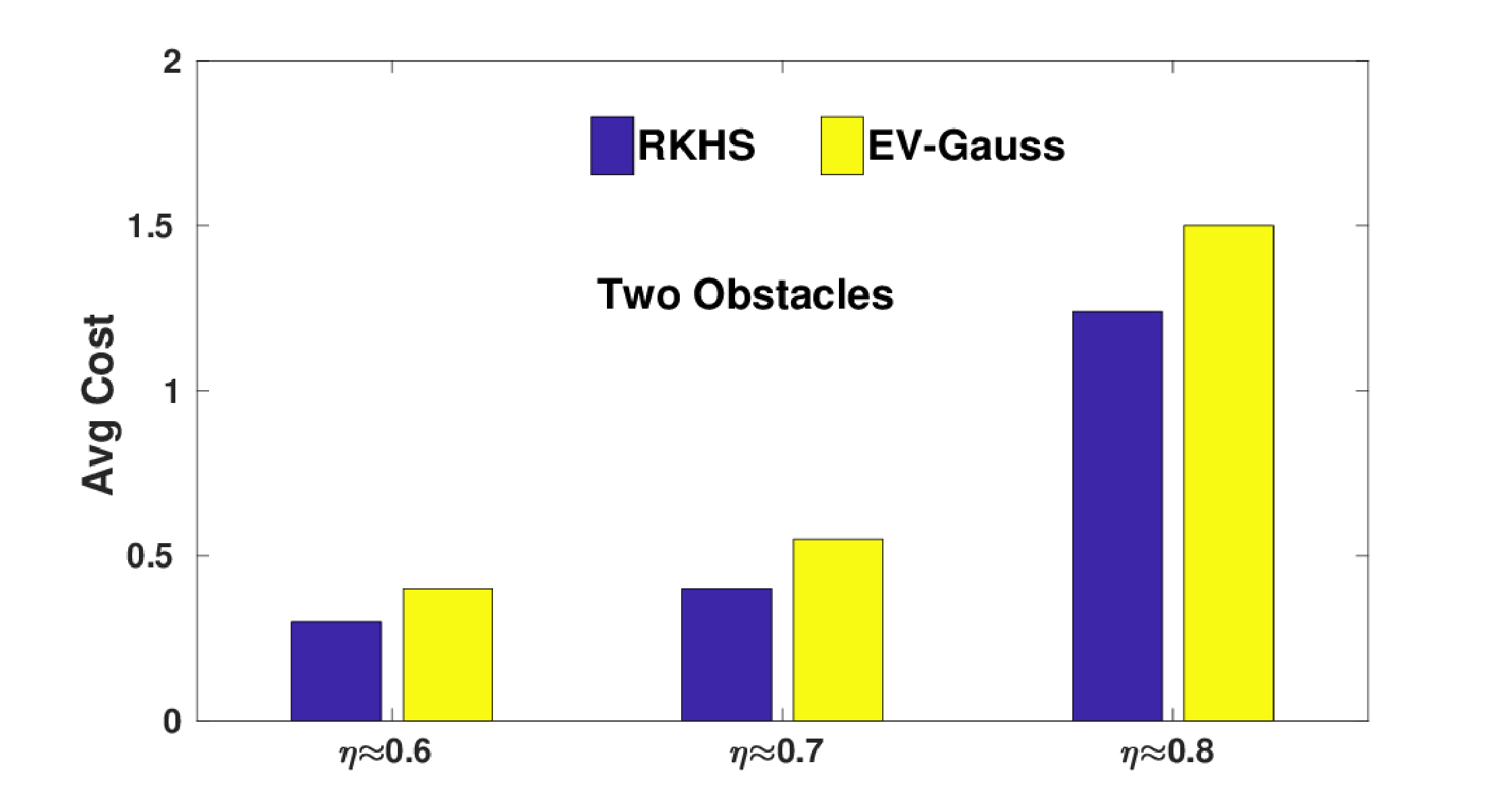 (b)
(b)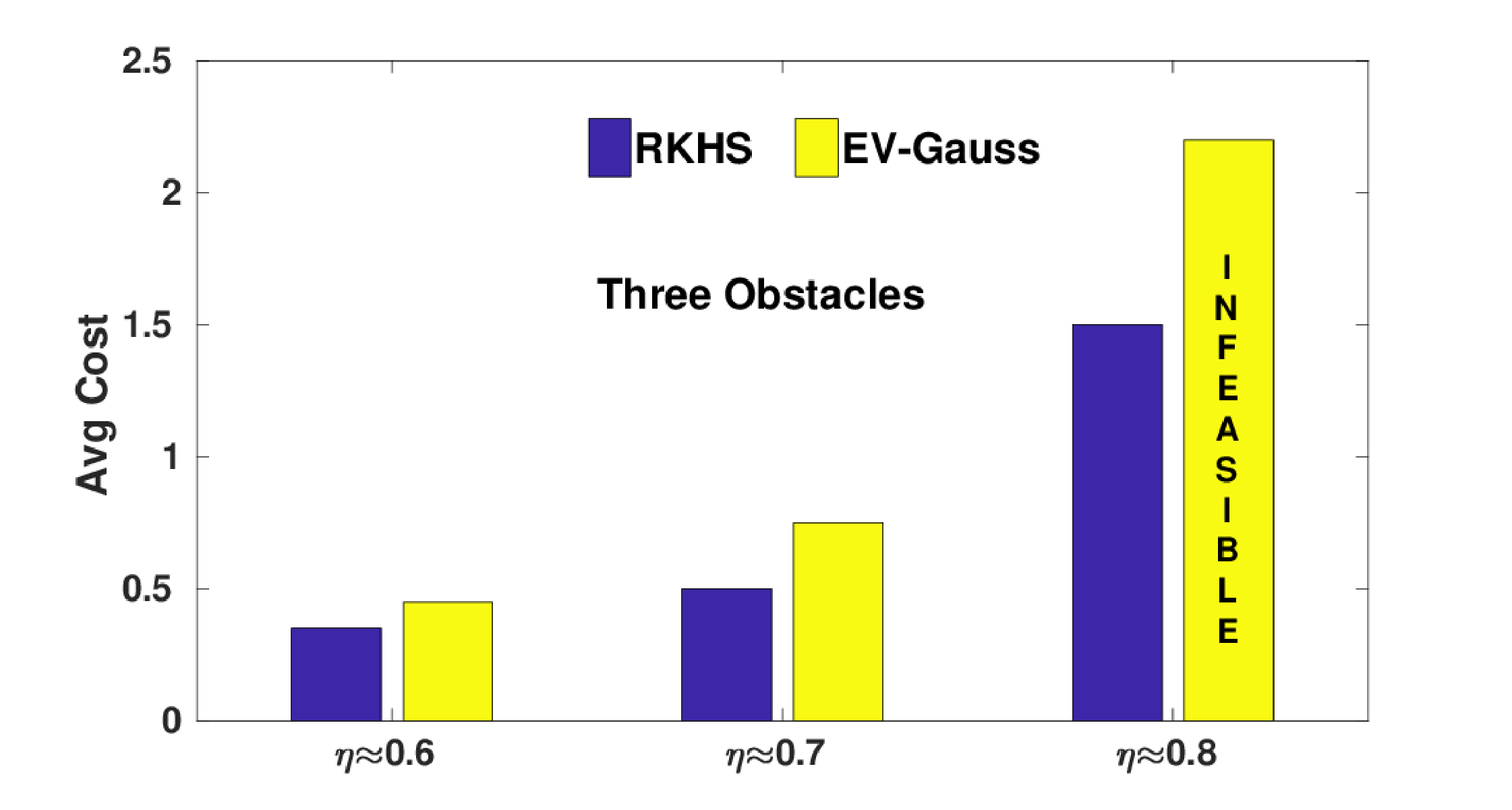 (c)
(c)Average cost obtained with our RKHS based algorithm and EV-Gauss. At \( \eta=0.80 \), EV-Gauss often resulted in infeasible solutions; The last figure (from the left) highlights this fact.